Overview
The CLASS Cosmology object
Although the main pyRSD modules require the use of the main
pyRSD.rsd.cosmology.Cosmology class, the pyRSD.pygcl module
relies on the pyRSD.pygcl.Cosmology class. A
pyRSD.pygcl.Cosmology object can be easily initialized
from a pyRSD.rsd.cosmology.Cosmology object via the
to_class() function, as
In [1]: from pyRSD.rsd.cosmology import Planck15

In [2]: from pyRSD import pygcl

In [3]: class_cosmo = Planck15.to_class()

In [4]: print(class_cosmo)
<pyRSD.pygcl.Cosmology; proxy of <Swig Object of type 'Cosmology *' at 0x7f3f0e776bd0> >
Computing Background Quantities
The pyRSD.pygcl.Cosmology calls the CLASS code to compute various
cosmological parameters and background quantities as a function of redshift
See the API for the full list of available quantities
that CLASS can compute. For example, to compute the growth rate as a
function of redshift
In [5]: z = numpy.linspace(0, 3, 100)

In [6]: growth = class_cosmo.f_z(z)
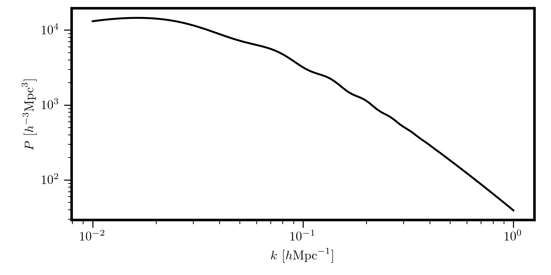
The Linear Power Spectrum
Most importantly for pyRSD, the pyRSD.pygcl module includes
functionality to compute the linear matter power spectrum using CLASS.
The main object for this calculation is the pyRSD.pygcl.LinearPS
class, which can be initialized as
# initialize at z = 0
Plin = pygcl.LinearPS(class_cosmo, 0)

# renormalize to different SetSigma8AtZ
Plin.SetSigma8AtZ(0.62)

# evaluate at k
k = numpy.logspace(-2, 0, 100)
Pk = Plin(k)

# plot
plt.loglog(k, Pk, c='k')
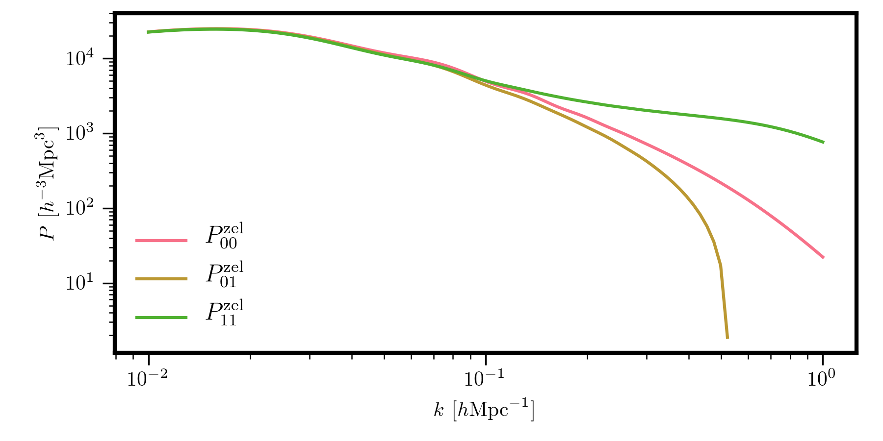
Zel’dovich Power Spectra
The pyRSD.pygcl module can also be used to directly compute
power spectra in the Zel’dovich approximation. For example,
# density auto power
P00 = pygcl.ZeldovichP00(class_cosmo, 0)

# density - radial momentum cross power
P01 = pygcl.ZeldovichP01(class_cosmo, 0)

# radial momentum auto power
P11 = pygcl.ZeldovichP11(class_cosmo, 0)

# plot
k = numpy.logspace(-2, 0, 100)
plt.loglog(k, P00(k), label=r'$P_{00}^\mathrm{zel}$')
plt.loglog(k, P01(k), label=r'$P_{01}^\mathrm{zel}$')
plt.loglog(k, P11(k), label=r'$P_{11}^\mathrm{zel}$')
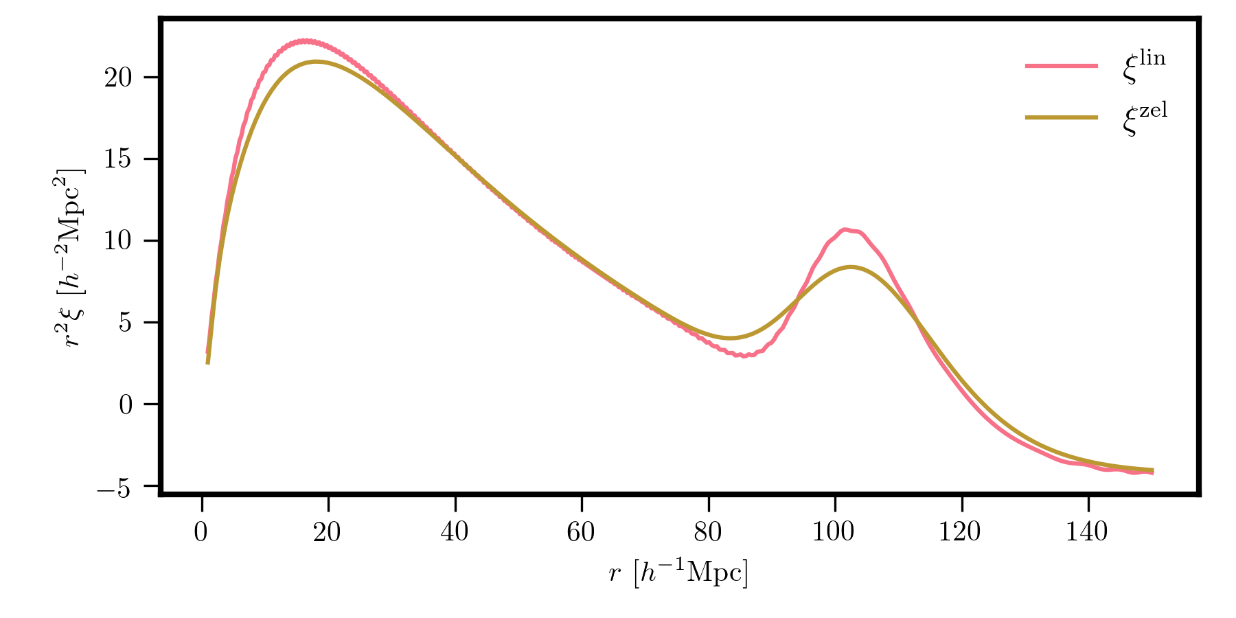
The Correlation Function
The pyRSD.pygcl module also includes functionality for computing
the linear and Zel’dovich correlation functions. This is computed by
taking the Fourier transform of the power spectrum using FFTLog.
# linear correlation function
CF = pygcl.CorrelationFunction(Plin)

# Zeldovich CF at z = 0.55
CF_zel = pygcl.ZeldovichCF(class_cosmo, 0.55)

# plot
r = numpy.logspace(0, numpy.log10(150), 1000)
plt.plot(r, r**2 * CF(r), label=r'$\xi^\mathrm{lin}$')
plt.plot(r, r**2 * CF_zel(r), label=r'$\xi^\mathrm{zel}$')