Quickstart
The pyRSD package provides a number of examples in order to get users
up and running quickly. Once these examples have been downloaded, the
user can start running their own parameter fits using the example data
and parameter files. The executable responsible for downloading the pyRSD
examples is pyrsd-quickstart, which has the following calling sequence:
$ pyrsd-quickstart -h
usage: pyrsd-quickstart [-h]
                        {galaxy/survey-poles,galaxy/periodic-poles,galaxy/periodic-pkmu}
                        dirname

download example data and parameter files to get up and running with pyRSD

positional arguments:
  {galaxy/survey-poles,galaxy/periodic-poles,galaxy/periodic-pkmu}
                        which example to download
  dirname               the output directory to save the downloaded files; if
                        it doesn't exist it will be created

optional arguments:
  -h, --help            show this help message and exit
The first argument provided to the command is the name of the example to download, which should be of the following:
| Example Name | Description |
| galaxy/periodic-pkmu | Fitting \(P(k,\mu)\) galaxy data from a periodic box simulation |
| galaxy/periodic-poles | Fitting \(P_\ell(k)\) galaxy data from a periodic box simulation |
| galaxy/survey-poles | Fitting \(P_\ell(k)\) galaxy data from a simulation with a realistic survey window function |
And the second argument is the name of the directory to download the files too.
So, for example, to download the files from the periodic-poles examples to
a directory called pyRSD-example simply do
pyrsd-quickstart galaxy/periodic-poles pyRSD-example
Running Parameter Fits
With the example downloaded, the user can run MCMC or nonlinear optimization
fits using the default model parametrization with the rsdfit command.
See The Free Parameters for a table of the default free parameters and
The Constrained Parameters for a table of the default constrained parameters.
For example, to run 10 nonlinear optimization steps (using the LBFGS optimization algorithm), you can do
rsdfit nlopt -m pyRSD-example/model.npy -p pyRSD-example/params.dat -o pyRSD-example-results -i 10
or to run 10 MCMC iterations (using 30 emcee walkers), you can do
rsdfit mcmc -m pyRSD-example/model.npy -p pyRSD-example/params.dat -o pyRSD-example-results -i 10 -w 30
The number of iterations has been set to 10 here just for illustration purporse. Typically, the LBFGS algoritm will take \(\sim100-200\) steps to converge, and the mcmc algorithm will need 1000s of iterations to fully explore the posterior distributions of the parameters.
Analyzing the Fit Results
The rsdfit saves the best-fit parameter set to a numpy .npz file in
the directory specified via the -o output, which is pyRSD-example-results
in the example above. There are two Python objects in pyRSD that can read these
files, depending on the type of fit that was run. For mcmc fits, use the
pyRSD.rsdfit.results.EmceeResults class and for nlopt fits, use
the pyRSD.rsdfit.results.LBFGSResults class.
For example, to explore the fitting results from a mcmc fit
In [1]: from pyRSD.rsdfit.results import EmceeResults, LBFGSResults

In [2]: mcmc_results = EmceeResults.from_npz('mcmc_result.npz')

# print out a summary of the parameters, with mean values and 68% and 95% intervals
In [3]: print(mcmc_results)
Free parameters [ median (+/-68%) (+/-95%) ]
_______________
<Parameter Nsat_mult:      2.423 (+0.2082 -0.1809) (+0.4361 -0.3432)>
<Parameter alpha_par:      1.009 (+0.00682 -0.007681) (+0.01353 -0.01379)>
<Parameter alpha_perp:     1.005 (+0.004241 -0.004049) (+0.008281 -0.008406)>
<Parameter b1_cA:          1.999 (+0.05749 -0.05801) (+0.1126 -0.1265)>
<Parameter f:              0.867 (+0.02897 -0.02502) (+0.05642 -0.05073)>
<Parameter f1h_sBsB:       3.569 (+0.5521 -0.6841) (+1.224 -1.396)>
<Parameter fs:             0.1434 (+0.007553 -0.008046) (+0.01554 -0.01544)>
<Parameter fsB:            0.4662 (+0.08146 -0.0792) (+0.1685 -0.1606)>
<Parameter gamma_b1sA:     1.31 (+0.1001 -0.1032) (+0.2119 -0.2205)>
<Parameter gamma_b1sB:     2.343 (+0.1661 -0.181) (+0.3225 -0.3636)>
<Parameter sigma8_z:       0.5411 (+0.01224 -0.01362) (+0.02611 -0.02452)>
<Parameter sigma_c:        0.9297 (+0.06205 -0.06473) (+0.1126 -0.1177)>
<Parameter sigma_sA:       3.443 (+0.2779 -0.2702) (+0.5436 -0.5378)>

Constrained parameters [ median (+/-68%) (+/-95%) ]
______________________
<Parameter NsBsB:          5.178e+04 (+1.721e+04 -1.36e+04) (+4.16e+04 -2.44e+04)>
<Parameter b1_sA:          2.617 (+0.169 -0.1761) (+0.3037 -0.3725)>
<Parameter sigma_sB:       5.71 (+0.3067 -0.2659) (+0.6624 -0.4928)>
<Parameter NcBs:           2.261e+04 (+2900 -2096) (+6130 -4001)>
<Parameter b1_sB:          4.686 (+0.2679 -0.3235) (+0.5596 -0.672)>
<Parameter b1_cB:          3.175 (+0.1504 -0.1736) (+0.2942 -0.3522)>
<Parameter fcB:            0.122 (+0.01336 -0.0149) (+0.02856 -0.02761)>
<Parameter b1_c:           2.141 (+0.04721 -0.04684) (+0.08834 -0.08337)>
<Parameter b1:             2.344 (+0.05369 -0.04764) (+0.1051 -0.1053)>
<Parameter fsigma8:        0.4689 (+0.009673 -0.009076) (+0.01866 -0.01848)>
<Parameter b1_s:           3.575 (+0.1907 -0.2037) (+0.3854 -0.4186)>
<Parameter alpha:          1.006 (+0.004107 -0.004331) (+0.007706 -0.0083)>
<Parameter epsilon:        0.00125 (+0.002298 -0.002462) (+0.004696 -0.004652)>
<Parameter b1sigma8:       1.268 (+0.007575 -0.008006) (+0.01531 -0.01495)>
<Parameter F_AP:           1.004 (+0.006927 -0.007386) (+0.01419 -0.01393)>

# access parameters like a dictionary
In [4]: fsat = mcmc_results['fs']

In [5]: print(fsat.median)
0.14339263725236592
and to explore the fitting results from a nlopt fit
In [6]: nlopt_results = LBFGSResults.from_npz('nlopt_result.npz')

# print out a summary of the parameters, with best-fit values
In [7]: print(nlopt_results)
minimum chi2 = 120.57745038002743

Free parameters [ mean ]
_______________
Nsat_mult      : 2.4324089012014207
alpha_par      : 1.0072991239946898
alpha_perp     : 1.0048333693698863
b1_cA          : 2.0068377074748778
f              : 0.8735346371321935
f1h_sBsB       : 3.6140366462767153
fs             : 0.14175570928456935
fsB            : 0.4782779433107577
gamma_b1sA     : 1.31213984320964
gamma_b1sB     : 2.3651886897525896
sigma8_z       : 0.5363993024676117
sigma_c        : 0.9194602113178405
sigma_sA       : 3.420304679802984

Constrained parameters [ mean ]
_________________________
NsBsB          : 51736.1
b1_sA          : 2.6332517
NcBs           : 23183.68
fcB            : 0.11864934
sigma_sB       : 5.739127
b1_sB          : 4.74655
b1_cB          : 3.2117057
epsilon        : 0.0008172965
b1_c           : 2.1497946
b1sigma8       : 1.2667638
alpha          : 1.0056546
F_AP           : 1.0024539
b1_s           : 3.6439955
fsigma8        : 0.46856338
b1             : 2.3616061

# access best-fit values like a dictionary
In [8]: fsat = nlopt_results['fs']

In [9]: print(fsat)
0.14175570928456935
Comparing the Best-fit Model to Data
Users can compare the best-fitting model to the data by loading the
results of a fitting run using the pyRSD.rsdfit.FittingDriver.
We can easily initialize this object by passing the directory where the results
were written to the pyRSD.rsdfit.FittingDriver.from_directory function.
For the example data downloaded above, we can explore both the data
and theory simulataneously using the included result file
nlopt_result.npz:
from pyRSD.rsdfit import FittingDriver

# load the model and results into one object
d = FittingDriver.from_directory('pyRSD-example', model_file='pyRSD-example/model.npy', results_file='pyRSD-example/nlopt_result.npz')

# set the fit results
d.set_fit_results()

# the best-fit log probability (likelihood + priors)
print(d.lnprob())

# the best-fit chi2
print(d.chi2())

# the best-fit reduced chi2
print(d.reduced_chi2())

# make a plot of the data vs the theory
d.plot()
show()
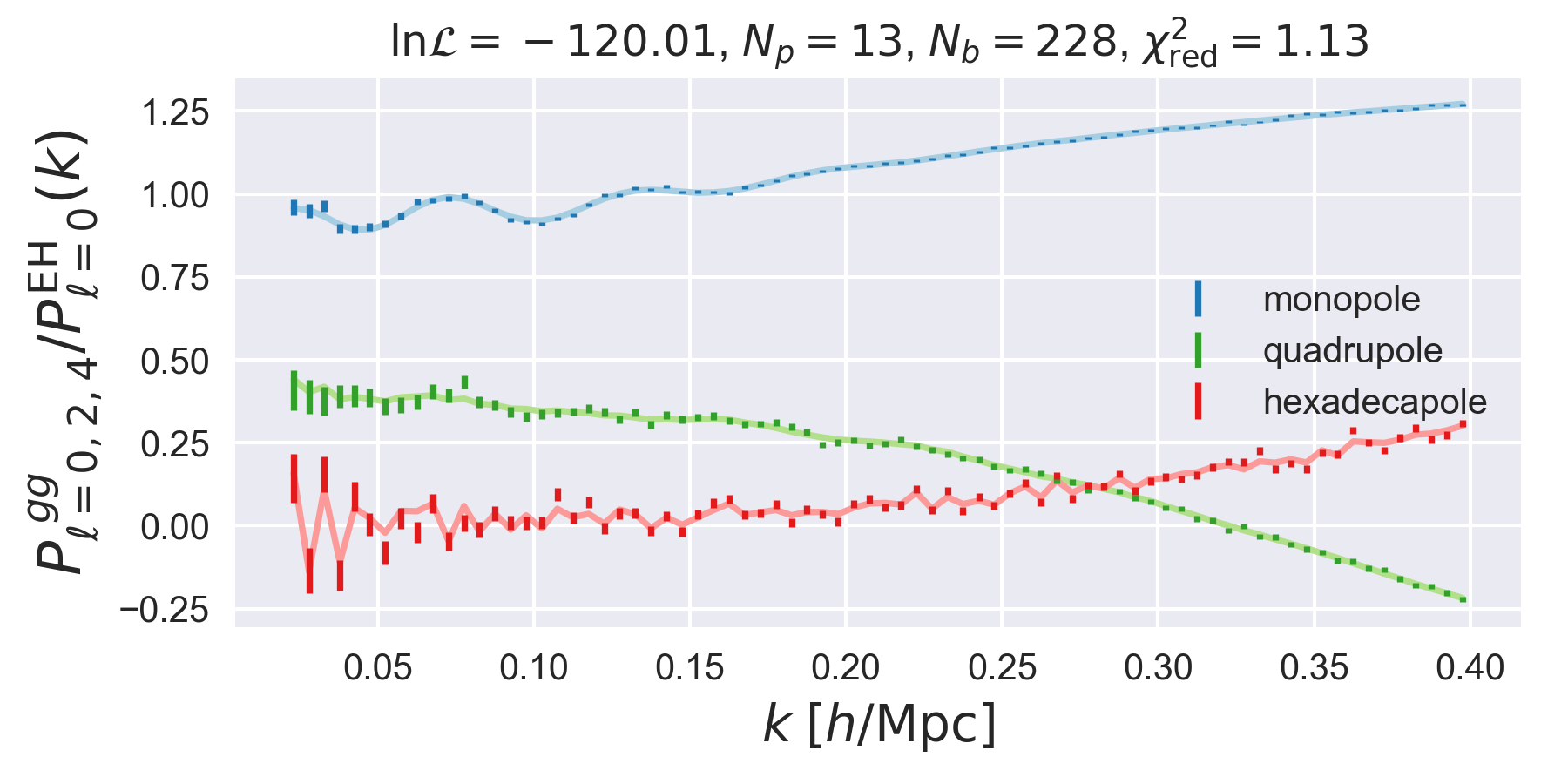
In this plot, we show the monopole, quadrupole, and hexadecapole normalized
by the smooth, no-wiggle Eisenstein and Hu
monopole. All of the above steps are identical if we are analyzing \(P(k,\mu)\)
data rather than \(P_\ell(k)\) data. For example, if the periodic-pkmu
example is downloaded, running the function FittingDriver.plot() using
the included result file nlopt_result.npz produces the following figure:
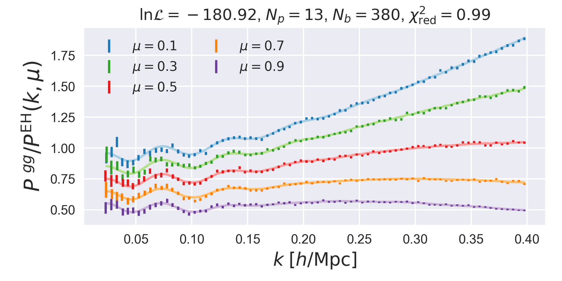
This plot shows the best-fit theory and data for 5 wide \(\mu\) bins, normalized by the linear Kaiser \(P(k,\mu)\), using the no-wiggle Eisenstein and Hu linear power spectrum.